1. Introduction
What does it mean for a neural network to understand a shape?
When we look at a chair, we don’t perceive a list of coordinates. We perceive surfaces, curvature, the way light catches an edge. Classical deep learning sidesteps this question by projecting 3D objects onto 2D grids — depth maps, multi-view renders — and applying convolutions designed for images. It works, but something is lost in translation.
Point clouds offer a more honest representation: a set of 3D coordinates sampled directly from an object’s surface, with no forced projection, no grid, no privileged orientation. But they come with their own challenge — there is no natural ordering to a set of points, and standard neural network operations assume exactly that.
Geometric machine learning is the field that takes this challenge seriously. Rather than forcing geometric data into Euclidean templates, it asks a more interesting question: what mathematical structure does the data actually have, and how do we build models that respect it?
In this post we build a complete pipeline — procedural dataset generation, a PointNet classifier, and a desktop viewer — and use it to explore one concrete instance of that question: what happens when we stop treating surface normals as plain features, and start recognising them as sections of the tangent bundle?
The answer, as we will see, is both practically measurable and geometrically instructive.
2. A Brief Geometry Detour: Fiber Bundles
Imagine the surface of a sphere. At every point, you can place a flat plane that just touches the sphere at that point — the tangent plane. Do this at every point simultaneously, and you get a family of planes indexed by the surface itself. That family is the tangent bundle.
More formally: given a smooth manifold M (our surface), the tangent bundle TM is a new space that pairs each point p ? M with its tangent space T_pM — the space of all directions in which you can move along the surface from p. The tangent bundle is itself a manifold, of twice the dimension of M.
A fiber bundle generalises this idea. Instead of tangent spaces, you attach an arbitrary space F — the fiber — to each point of M. The result is a space that locally looks like M × F, but may be globally twisted. The tangent bundle is simply the special case where F = T_pM.
So where do surface normals fit in?
At each point of a smooth surface embedded in R³, the unit normal is a vector perpendicular to the tangent plane. It is not an element of the tangent bundle — it lives in the normal bundle, the complementary one-dimensional fiber at each point. But crucially, it encodes the same local geometric information: knowing the normal is equivalent to knowing the orientation of the tangent plane.
This is the key distinction that matters for machine learning. When we append surface normals to our XYZ coordinates and feed them as a flat 6D vector to a neural network, we are technically correct — but geometrically naive. We are ignoring the fact that positions and normals transform differently. Under a rigid motion of the object, positions translate and rotate, while normals only rotate — they are insensitive to translation because they are direction vectors, not position vectors. A model that truly understands this structure should encode it explicitly, not leave it for the network to discover from data.
In our pipeline, we take a first step in this direction: when we apply a random rotation during data augmentation, we apply the same rotation matrix to both the XYZ coordinates and the surface normals. This is not optional — it is the geometrically correct thing to do, and getting it wrong would corrupt the relationship between a point and its normal. It is a small thing, but it is precisely the kind of constraint that separates geometric machine learning from plain machine learning applied to geometric data.
3. The Dataset: Procedural 3D Objects
Before training anything, we need data. Rather than downloading an existing benchmark, we generate our own — which turns out to be both instructive and practical.
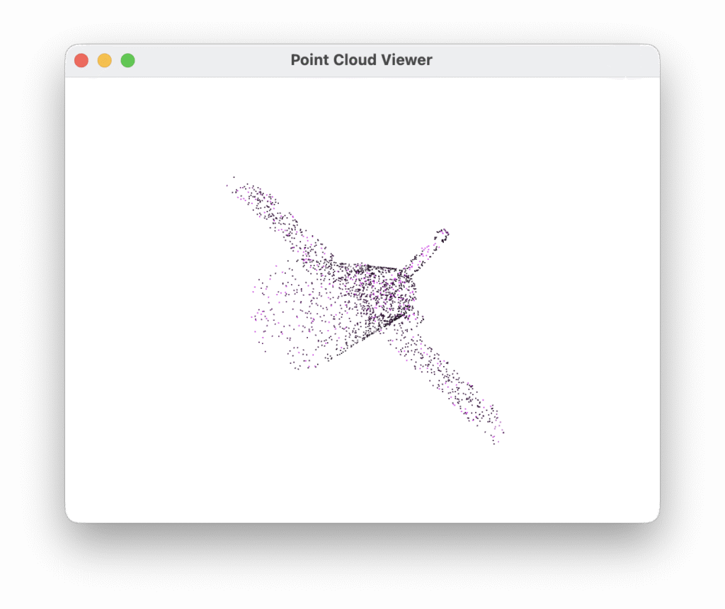
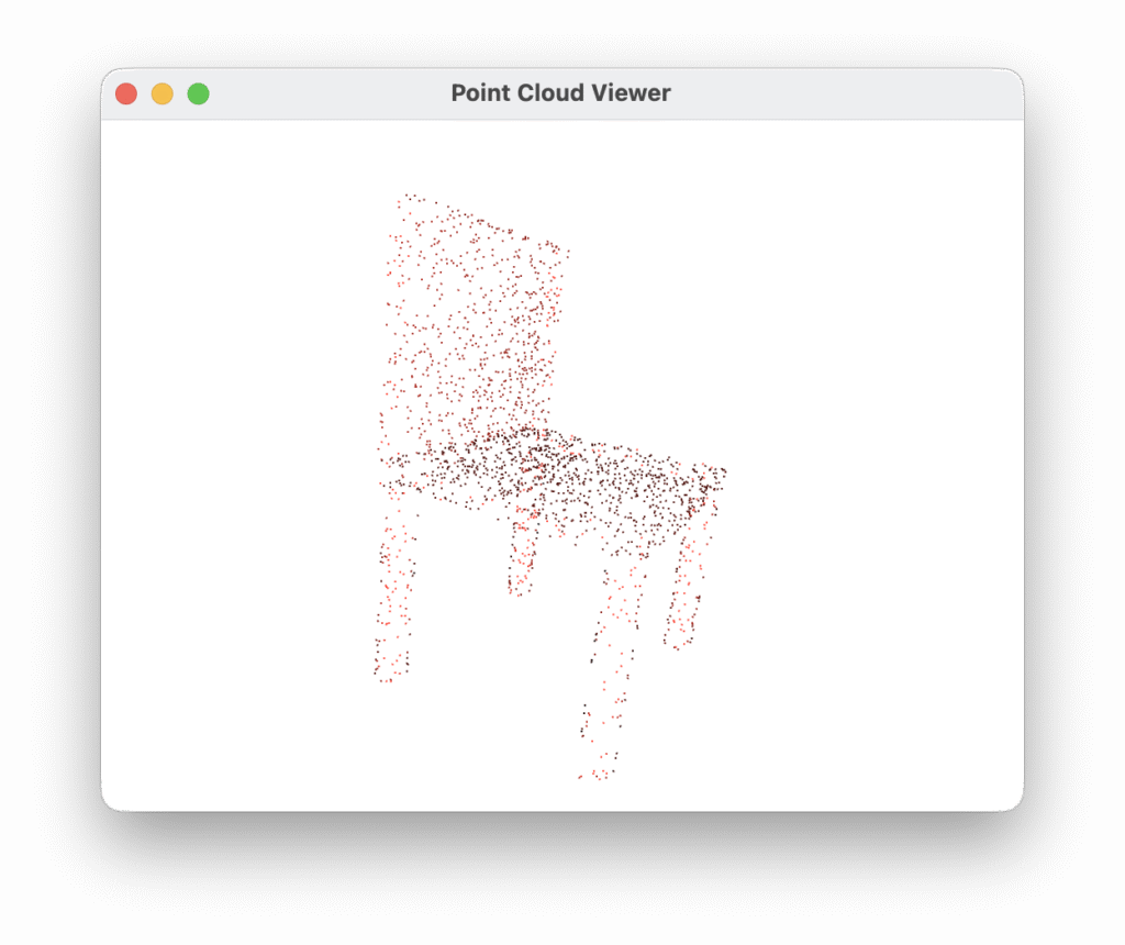
The dataset consists of ten object classes: airplane, bookshelf, bottle, car, chair, lamp, monitor, mug, sofa, and table. Each object is built procedurally from geometric primitives — boxes, cylinders, cones, spheres — assembled with randomised proportions. A chair, for instance, is a seat box, a backrest, and four cylindrical legs, each with independently sampled dimensions. This means no two instances of the same class are identical, while the overall shape remains recognisable. One hundred instances per class are generated, split 80/20 into training and test sets.
Points are sampled uniformly from mesh surfaces using trimesh, which also provides face normals at each sample location — precisely the tangent bundle information discussed in the previous section. Each cloud contains 2048 points, stored as a binary PLY file with six properties per vertex: x y z nx ny nz.
Generating data synthetically offers a significant advantage for experimentation: we control every variable. There is no sensor noise, no missing data, no class imbalance, no licensing ambiguity. The dataset is a clean baseline — a controlled environment in which the effect of adding geometric structure can be measured directly, without confounding factors.
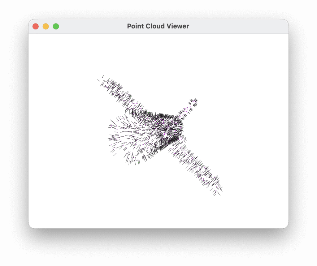
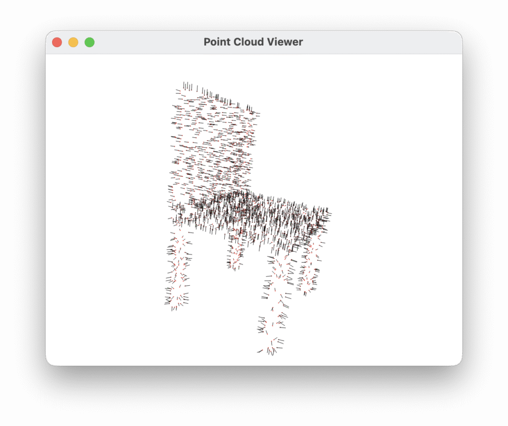
A desktop viewer built on Open3D lets you browse the dataset interactively, with each class rendered in a distinct colour. Pressing V toggles the display of surface normal vectors — a useful sanity check that the normals are geometrically consistent with the underlying shape.
4. PointNet: Deep Learning on Unordered Sets
The central challenge of learning on point clouds is that a set has no canonical order. Shuffle the 2048 points in any cloud and you have the same object — but a naive neural network would treat the two orderings as completely different inputs. Any architecture that takes point clouds seriously must be permutation invariant by design, not by accident.
PointNet, introduced by Qi et al. in 2017, solves this with an elegant observation: if you apply the same function independently to each point and then aggregate the results with a symmetric operation, the output is guaranteed to be order-independent. In practice, the function is a shared MLP — the same weights applied to every point — and the symmetric operation is a global max pooling across all points. Each dimension of the resulting 1024-dimensional vector captures the most prominent activation for that feature across the entire cloud, regardless of how the points are ordered.
The architecture goes further with two T-Nets — small networks, each structured like a miniature PointNet, that regress a transformation matrix rather than a class label. The first T-Net operates on raw input coordinates and produces a 6×6 matrix (6×6 because normals are included) that rigidly aligns the point cloud before any learning takes place. The second operates in feature space and produces a 64×64 matrix that aligns the learned representations. Both can be thought of as learned canonicalization steps: the network figures out, from the data itself, which orientation makes classification easiest.
The 64×64 feature transform introduces a subtlety: an unconstrained 64×64 matrix has far too many degrees of freedom, and the optimiser can easily find degenerate solutions. To prevent this, the original paper adds a regularisation term to the loss that penalises deviation from orthogonality:
\({L}_{\text{reg}} = \lambda \cdot \left\| \mathbf{I} – A A^{\top} \right\|_F^2\)
This encourages the learned transform to behave like a rotation — preserving distances and angles in feature space — without hard-constraining it. In our implementation lambda = 0.001, following the original paper.
The full classification head takes the 1024-dimensional global descriptor and passes it through three fully connected layers (512 -> 256 -> num_classes), with batch normalization, ReLU activations, and dropout after each of the first two. The result is a model with 3.4 million parameters that trains comfortably on a laptop GPU in a matter of minutes.
5. Plugging in the Fiber Bundle
So far we have a clean dataset and a solid architecture. The question is: what exactly changes when we move from raw XYZ coordinates to XYZ plus surface normals — and does the geometry actually matter, or is it just six numbers instead of three?
The practical change is straightforward. During dataset generation, trimesh provides face normals at every sampled point as a by-product of the surface sampling process. We store them alongside the coordinates in the PLY file as nx ny nz, giving a 6D descriptor per point. On the model side, the input T-Net grows from 3×3 to 6×6, and the first shared MLP layer accepts six channels instead of three. Everything else in the architecture remains identical.
But the interesting part is not the change in dimensionality — it is the constraint we impose during augmentation.
When we apply a random rotation to a point cloud during training, we sample a matrix R is an element of SO(3) and apply it to the XYZ coordinates. What should we do with the normals? A surface normal is not a position — it is a direction vector attached to the surface, a local encoding of how the surface is oriented in space. Under a rigid motion of the object, it must rotate exactly as the surface rotates. Translating the object leaves the normals unchanged; rotating the object rotates the normals by the same R.
This means the correct augmentation is:
cloud[:, :3] = (R @ cloud[:, :3].T).T   # rotate positions
cloud[:, 3:] = (R @ cloud[:, 3:].T).T   # rotate normals — same R
Applying a different rotation to the normals, or worse, leaving them unrotated while rotating the positions, would silently corrupt the geometric relationship between a point and its normal. The network would receive inconsistent data, and any signal carried by the normals would be buried in noise. This is precisely the kind of error that is easy to make and hard to debug — the code runs, the loss decreases, but the model learns something slightly wrong.
Getting this right is a concrete instance of the broader principle behind geometric machine learning: the structure of the data — here, the fact that normals are sections of the normal bundle and must transform covariantly with the base manifold — should be reflected explicitly in how we process it, not left as something the network might eventually infer.
The empirical result is immediate. Comparing two identical training runs — same architecture, same hyperparameters, same random seed, same three epochs — the only difference being the presence or absence of normals:
| Input | Val accuracy @ epoch 3 |
|---|---|
| XYZ only | 71% |
| XYZ + normals | 78% |
Seven percentage points of improvement, for free, from a geometrically correct augmentation and an honest representation of the data’s structure.
It is worth pausing on what this number does and does not tell us. PointNet is not a bundle-aware architecture — it treats the 6D input as a flat vector and has no explicit mechanism for respecting the covariance between positions and normals beyond what the T-Net can learn. The improvement comes from giving the network more information, not from giving it a better inductive bias. A truly geometry-aware model — one that builds the transformation laws of the tangent bundle directly into its layers — would extract even more signal from the same data.
6. What This Opens Up
The results we have seen are encouraging, but it is worth being honest about what we have and have not achieved.
PointNet with surface normals is not a bundle-aware architecture. The 6×6 input T-Net learns a linear transformation of the joint (position, normal) space, but it has no explicit knowledge that the first three dimensions and the last three are geometrically coupled — that rotating one necessarily rotates the other. We enforce this coupling in the data augmentation, but the model itself is free to ignore it. What we have built is a geometrically informed pipeline, not a geometrically equivariant one.
The distinction matters. A truly equivariant model would guarantee, by construction, that rotating the input produces a predictably rotated internal representation — not approximately, not on average, but exactly, for every input and every rotation. This is the property that makes a model genuinely aware of geometric structure rather than merely exposed to it.
This is precisely where the field is heading, and where the most interesting current research lives.
PointNet++ takes a first step by introducing a hierarchical structure — local neighbourhoods are processed before global aggregation, giving the model a sense of spatial scale. Surface normals become more useful here because local geometry is where they carry the most information.
DGCNN (Dynamic Graph CNN) constructs a graph in feature space at each layer and applies graph convolutions. The graph changes as features evolve, allowing the model to dynamically redefine what “local” means. Normals can seed the initial graph with geometrically meaningful edges.
DiffusionNet operates intrinsically on the surface manifold itself, using heat diffusion as the aggregation operator. It is largely invariant to how the surface is discretised — as a mesh, a point cloud, or otherwise — and handles surface normals naturally as part of the manifold structure.
Gauge Equivariant CNNs and DeltaConv go furthest in the direction suggested by our fiber bundle framing. They define convolution filters that are equivariant with respect to local rotations of the tangent frame — the gauge group of the tangent bundle. In these architectures, the coupling between positions and normals is not something we need to enforce manually in augmentation: it is baked into the mathematics of the convolution itself.
The progression from PointNet to these architectures is not merely a sequence of accuracy improvements. It is a conceptual journey from treating geometric data as a bag of vectors, to treating it as a sampled manifold with intrinsic structure, to building models whose symmetries match the symmetries of the data by construction. Each step requires taking the geometry more seriously — and each step rewards that seriousness with models that generalise better, require less data, and are more interpretable.
Our pipeline is a starting point. The dataset format, the training loop, and the evaluation infrastructure are all designed to accommodate more sophisticated architectures. Swapping PointNet for any of the models above requires changing only src/model.py — everything else stays the same.
7. Code & Conclusion
All the code described in this post is available on GitHub. The repository is self-contained and requires only a Python virtual environment to run.
# Clone and set up
git clone https://github.com/your-username/point-cloud-gen.git
cd point-cloud-gen
python -m venv venv && source venv/bin/activate
pip install -r generator/requirements.txt
pip install -r classifier/requirements.txt

# Generate the dataset (100 clouds per class, 2048 points each)
python generator/generate.py --seed 42

# Browse it interactively (N = next, P = prev, V = normals, Q = quit)
python generator/viewer.py

# Train
python classifier/train.py --seed 42 --run-name exp01

# Evaluate
python classifier/evaluate.py --run-dir experiments/exp01
The project is structured in two independent modules — generator/ and classifier/ — sharing only the data/ directory at the root. This separation is intentional: the dataset is a first-class artifact, not a side effect of training. As the classifier evolves toward more sophisticated architectures, the dataset stays fixed, making results comparable across experiments.
8. Final thoughts
We started with a question: does it matter how we represent geometric data, or is a neural network flexible enough to figure it out regardless?
The answer, as always in machine learning, is nuanced. A network can learn a great deal from raw coordinates alone. But when we take the geometry seriously — sampling normals from the tangent bundle, rotating them equivariantly during augmentation, feeding a 6D descriptor that honestly encodes both position and local surface orientation — the model learns faster and more accurately, with no additional architectural complexity.
This is the central promise of geometric machine learning: not that geometry replaces learning, but that the right geometric representation makes learning easier, more data-efficient, and more principled. Surface normals are a mild example of this principle. Gauge equivariant convolutions are a deeper one. The underlying idea is the same: structure in the data, when respected by the model, is never wasted.
The tangent bundle is a good place to start. It is the simplest fiber bundle, the one closest to our intuitions about surfaces and directions, and the one most immediately accessible through standard tools like trimesh and PyTorch Geometric. From here, the path toward intrinsic convolutions, equivariant architectures, and genuine manifold-aware learning is a natural progression — not a leap into abstraction, but a series of steps, each grounded in the geometry of the previous one.
9. Download the Complete Code
The complete code is available at GitHub. This program is written using Claude Code Desktop on Mac with Sonnet 4.6 as model.
These materials are distributed under MIT license; feel free to use, share, fork and adapt these materials as you see fit.
Also please feel free to submit pull-requests and bug-reports to this GitHub repository or contact me on my social media channels available on the contact page.
10. References & Further Reading
BibTeX
@inproceedings{qi2017pointnet,
  title     = {PointNet: Deep Learning on Point Sets for 3D Classification and Segmentation},
  author    = {Qi, Charles R. and Su, Hao and Mo, Kaichun and Guibas, Leonidas J.},
  booktitle = {Proceedings of the IEEE Conference on Computer Vision and Pattern Recognition (CVPR)},
  pages     = {652--660},
  year      = {2017}
}
APA
Qi, C. R., Su, H., Mo, K., & Guibas, L. J. (2017). PointNet: Deep learning on point sets for 3D classification and segmentation. Proceedings of the IEEE Conference on Computer Vision and Pattern Recognition (CVPR), 652–660.
arXiv